Convergence problems in (static) non-linear implicit finite element analyses can arise in any FE-solver, it is in general nothing specific for LS-DYNA. The reason for convergence problems is in many cases simply that finding static equilibrium in a non-linear FE analysis (involving contacts, material non-linearity possibly including material failure, and large deformations) is very difficult.
Here, some tips on how to identify and possibly circumvent convergence problems in implicit analyses in LS-DYNA are presented. Troubleshooting convergence problems is also treated in Appendix P of the Keyword Manual Vol I, and in Appendix C (Section 13) of the Guideline for implicit analyses.
A quick checklist for troubleshooting implicit convergence issues follows. Note that this is not a complete listing!
More details follows below in subsequent sections.
Information relevant for tracking convergence in LS-DYNA is printed in the d3hsp and the mes* files(s). It is recommended to set NLPRINT=3 on *CONTROL_IMPLICIT_SOLUTION in order to obtain detailed information on the progress of the convergence. Opening d3hsp in a text editor, it can look like this:
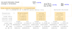
where we have highlighted the Line search information, the displacement norm, the energy norm and the force residual. Here DCTOL is the displacement relative convergence tolerance, ECTOL is the energy relative convergence tolerance and RCTOL is the residual force relative tolerance. Convergence is detected if all criteria are met, that is if the relative displacement norm is below DCTOL, the relative energy norm is below ECTOL and the relative residual force is below RCTOL. Alternatively, convergence may be detected based on an absolute criteria (a function of the model size and the tolerance ABSTOL). This helps in situations where residuals are small, for example if the model is just undergoing prescribed translation without any opposing forces. The tolerances are set by the keyword *CONTROL_IMPLICIT_SOLUTION.
Note that the node IDs and rigid body IDs where the residuals are the larges are printed. This can be very helpful information for localizing where in the model convergence problems originate.
The D3hsp View tool of LS-PrePost provides a convenient GUI for accessing the information in the d3hsp file (select Misc. from the top menu bar and then go to D3hsp View).

Convergence information can be accessed both in text form and as history plots of the norms. The nodes or rigid bodies with max residual values can be highlighted directly on the model.
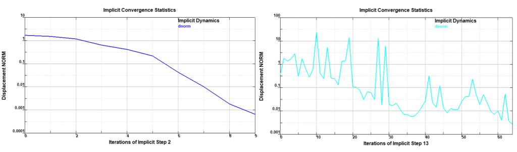
To classify the convergence behavior of the current simulation, it can be helpful to plot the relative displacement norm (Disp Norm, checked in the figure above). The left image of the figure below shows an example of very good convergence behavior: rapidly and monotonically decreasing norm, convergence within < 10 iterations. The right image shows an example of non-ideal convergence: the norm is “jumping up and down”, quite slowly decreasing, but convergence is obtained after 68 iterations. If this behavior occurs for many of the implicit time steps, it might be an indication that some kind of troubleshooting and model improvement is needed, even if Normal termination is obtained.
Reduce the risk for convergence problems by thorough model checking before submitting. Use the built-in tools of your preprocessor, for example in LS-PrePost, from the main menu bar select Application, and go to Model Checking and then General Checking.
In addition to the quality checking tools built into most preprocessors, LS-DYNA prints some general information on the mesh quality during initialization (from R14) in the d3hsp file. Search for the phrase “Listing the top “, for example
Listing the top 100 shell elements wrt aspect ratio
 ___________________________________________________
            Element #        Aspect ratio
            =========        ============
                    1    0.1965231305E+04
                  138    0.2857142857E+02
                15319    0.2857142857E+02
                15456    0.2857142857E+02
                  139    0.2714285714E+02
                  140    0.2714285714E+02
                  141    0.2714285714E+02
...
which indicates (in this example) that shell ID 1 probably needs fixing. A corresponding listing for solid elements will also be printed. The Warning 60421 will be issued for elements with nearly coincident nodes, for example
*** Warning 60421 (IMP+421)
    Solid element XX has a slightly bad edge/diag ratio,
    check if nodes are coincidental and adjust mesh.
The warning for bad Jacobian, for example,
*** Warning solid element # XX has a bad jacobian value -3.991E-01
is in general an indication that re-meshing is required.
Nodal projection by tied contacts may cause severely distorted elements, search for Warning 41240.
Direct connectivity between structural elements (shells, beams) and continuum elements can create mechanisms (like unintended joints or hinges) in the model, since the structural elements have nodal rotations, while the continuum elements have not. One example that may be problematic is if a spring element (*ELEMENT_BEAM, elform=6) is connected directly to one node of a solid element. Similar problems may arise when 6 DOF constraints are attached to only one 3 DOF node of a solid element. In some cases LS-DYNA will issue a warning for this, for example
 *** Warning 60301 (IMP+301)
     Using *CONSTRAINED_SPOTWELD with nodes without rotational dofs.
Care must be taken when connecting 1st and 2nd order elements by common nodes. Probably, tied contact is a better option.
Tied contacts are commonly used for creating connectivity between subassemblies, or connector entities (spotwelds, glue, etc.) in LS-DYNA. Use available tools to check that the tied contacts work as intended, for example in LS-PrePost: from the top menu bar, go to Application, then Model Checking > General Checking > Contact Check > Tied, and activate Show: Tied and Not Tied. This will highlight nodes that get tied in green, and missed nodes in red.
During initialization, LS-DYNA will issue warnings (in the mes0* file(s) ) for nodes not being tied, for example
*** Warning 50135 (MPP+135)
     Tracked node is not constrained
     since it is not found on a segment.

*** Warning 50136 (MPP+136)
     Tracked node is not constrained
     since it is too far from segment.
*** Warning 30455 (INI+455)
      Tied node # 267957 on the master side of surface # 100988
                 type # 7 also belongs to interface # 100987
                 tied constraint is released for node 31669
and from R14, the nodes that are not tied are collected in node sets, printed in the d3hsp file, for each tied contact ID, for example
untied *set_node_list below for interface ID 100987
*SET_NODE_LIST
    100987
     22924     23372     23376     23380     23384     23388     23392     23396
...
Some recommendations for defining tied contacts follow:
It is strongly recommended to use the Mortar contacts to model sliding contact in implicit analyses,
To start out with, use the default settings for contact stiffness. The use of contact damping (VDC on Card 2 of the contact definition) is not recommended for implicit analyses.
For the single surface Mortar contact, the option to disregard self-contact within a single part may be beneficial for convergence and performance. In many load cases for implicit analyses, buckling or severe deformation of parts is not expected, and then it is possibly to consider contact only part-to-part (not within the same part itself) by setting IGNORE=-2 on Optional Card C.
Use your preprocessing tools to check the model for unintended penetrations, for example in LS-PrePost, from the main top menu select Application, go to Model Checking, then General Checking and select Contact Check. Small initial penetrations are in many situations unavoidable, due to for example, discretization/facetting, and this type of penetrations are in most cases acceptable. Severe initial penetrations or intersections (like a part passing completely through another part) however can cause convergence problems, and such situations should (preferably) be resolved before submitting.
During initialization, the Mortar contact will print a detailed report of the initial penetrations in the mes* files, search for the phrase “Mortar contact information”. Before the first implicit step begins, the maximum penetration values for each contact definition are printed again in the mes* files, for example
  Contact sliding interface        151
    Number of contact pairs        80179
    Maximum penetration is  0.1686677E-17 between
    elements     515944 and     493946 on this processor
    Maximum relative penetration is  0.6337536E+00 % between
    elements     515944 and     493946 on this processor

BEGIN implicit dynamics step      1 t= 1.0000E-02             02/04/...
 ============================================================
It is good practice to check this initial report, to confirm that penetrations reported are in line with the expectations obtained from the checks in the preprocessor. If much bigger penetrations than expected are reported, one possible remedy could be to set IGNORE=-2 in case the contact is of single-surface type. If tetrahedral elements are involved, try specifying a reasonably small contact search depth by the PENMAX variable on Optional Card B.
In addition to the general recommendations for material models in implicit analyses, it may also be worth to carefully consider if failure criteria should be active in the model. It may be wise to first obtain a working model without failure, and once this is established try if also material failure is feasible. Element erosion can lead to severe convergence problems, but is possible to handle also in implicit analyses (or by automatically switching from implicit to explicit analysis). Material damage/failure defined by *MAT_ADD_{EROSION/DAMAGE_…} keywords can be deactivated globally, by setting MAEF=1 on *CONTROL_MAT.
This in general also applies to other failure types, for example *CONSTRAINED_JOINT_…_FAILURE.
Troubleshooting often is a process, involving several iterations, before a satisfactory solution can be found. It is about gathering information and consistently testing different hypotheses regarding what may be causing the problem.
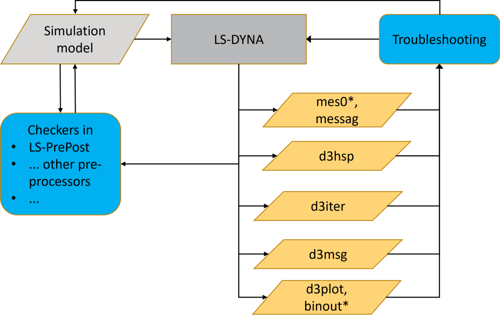
LS-DYNA will provide information that may be useful for troubleshooting in the ASCII text files
and in the binary databases (for 3D – visualization using for example, LS-PrePost)
The d3iter database may provide very useful information for troubleshooting, since it shows the deformed geometry after each nonlinear iteration (it may be required to use the displacement scale factor to discover where the “unexpected” deformations occur). It will also provide visual feedback if, for example, unconnected subassemblies are “flying away”.
The first step of troubleshooting is to establish a good starting point, with respect to control card settings, contacts etc. Follow the recommendations of Appendix P of the Keyword Manual, and the Guideline for implicit analyses in LS-DYNA. A brief summary follows:
An oscillating residual norm may be indication of a convergence problem caused by contacts. Track convergence norms in d3hsp and mes* – files, look for situations where one iteration is close to converge, the next norms are orders of magnitude higher, and then close to convergence again, and so on. The Mortar Contacts will also reject severely penetrated iterates, issuing an information message (search in d3hsp)
 Contact algorithm rejected current iterate,
 list of element pairs affected follows (at most 10):
     Element #           47052 vs           58986
 ------------------------------------------------------------
      automatic time step size DECREASE, RETRY step:
Here, the problematic element IDs are listed. Inspect the model (check d3plot and d3iter) in the vicinity of these elements and see if large deformations or penetrations can explain the behavior further.
Try to remove unintended initial penetration’s from the model. Use for example LS-PrePost to check and fix penetrations. Also check reported initial penetrations in the mes* files. In addition, by setting PENOUT=2 on *CONTROL_OUTPUT, it becomes possible to fringe plot absolute and relative penetrations in the d3plot file.
For intended penetrations (like press fit) use IGNORE = 3 or 4 of the Mortar contacts (or alternatively try *CONTACT_SURFACE_TO_SURFACE_INTERFERENCE_ID).
If you suspect that initial penetrations are spuriously found by the Mortar contacts, you could try
Contact release can cause severe convergence problems. Look for relative penetrations above 1, for example in the mes* file(s)
Maximum relative penetration is  0.1268843E+03 % between
     elements     162548 and     162861 on this processor
 *** Warning Penetration is close to maximum before release
In this case it would be a good idea to inspect the model in the vicinity of the element IDs 162548 and 162861. Increasing IGAP (to for eaxmple 5) on Optional Card C of the Mortar contact can reduce the risk for contact release.
One way to test if contact problems are causing the convergence problems can be to switch to tied contacts (*CONTACT_AUTOMATIC_…._MORTAR_TIED_ID) or reducing the contact stiffness (SFSA). Note that this is only a step in the investigations of the convergence problems, to see how the model responds to these changes, and it should not be seen as the final fix.
For high coefficients of friction, it can be beneficial for convergence to activate the unsymmetrical linear solver by setting LCPACK = 3 on *CONTROL_IMPLICIT_SOLVER.
A listing including some suggested actions follows.
*** Error 60004 (IMP+4)
    *********************************************************
    *                                                       *
    *                -  FATAL ERROR  -                      *
    *                                                       *
    *  Nonlinear solver failed to find equilibrium.         *
    *                                                       *
    *********************************************************
*** Error 60047 (IMP+47)
     *********************************************************
     *                                                       *
     *                    -  FATAL ERROR  -                  *
     *  AUTOSPC detected very large entries in the           *
     *  assembled matrix.  These are probably caused         *
     *  by overflow during elemental matrix computations.    *
     *  This could be caused by an energy explosion.         *
     *  Recommend switching to the REAL*8 version of LS-DYNA.*
     *                                                       *
     *********************************************************
*** Warning 60055 (IMP+55)
     *********************************************************
     *                                                       *
     *                -  WARNING  -                          *
     *                                                       *
     *          6 Unconstrained degrees of freedom have      *
     * been detected and removed from this IMPLICIT model.   *
     *                                                       *
     *********************************************************
*** Warning 60124 (IMP+124)
       2 negative eigenvalues detected
Convergence prevented due to unfulfilled bc...
Material model rejected current iterate,
list of elements affected follows (at most 20):

       Element # 26137

------------------------------------------------------------
automatic time step size DECREASE, RETRY step:
*** Error 60110 (IMP+110) (processor # 0)
     terminating : MF2 Factorization error 154
If the convergence problems prevail, it may be required to reduce the model in order to gain insight to the cause of the problems. Try removing parts, contacts, etc. to get a partial model working. Then add features again, step by step, to detect when the convergence problems appear again.
Things worth testing to see how the model reacts can be: